40 display data labels excel

Understand charts: Underlying data and chart representation (model ... Charts display data visually by mapping textual values on two axes: horizontal (x) and vertical (y). The x axis is called the category axis and the y axis is called the series axis. The category axis can display numeric as well as non-numeric values whereas the series axis only displays numeric values. SAS Tutorials: User-Defined Formats (Value Labels) Creating labels for each data value The most common way of labeling data is to simply assign each unique code its own label. Here, the format LIKERT_SEVEN assigns distinct labels to the values 1, 2, 3, 4, 5, 6, 7.

How to: Change the Display of Chart Axes - DevExpress Set the ChartTitleOptions.Visible property to true to display the axis title. To explicitly specify the text for the title, utilize the ChartText.SetValue method. Worksheet worksheet = workbook.Worksheets ["chartTask2"]; workbook.Worksheets.ActiveWorksheet = worksheet; // Create a chart and specify its location.

Display data labels excel

Excel Pivot Table tutorial - Ablebits To do this, in Excel 2013 and higher, go to the Insert tab > Charts group, click the arrow below the PivotChart button, and then click PivotChart & PivotTable. In Excel 2010 and 2007, click the arrow below PivotTable, and then click PivotChart. 3. Arranging the layout of your pivot table report › excel-chart-verticalExcel Chart Vertical Axis Text Labels • My Online Training Hub Note: I didn’t have the original data for Juan's chart so I’ve recreated by eye and as a result the lines in my chart are slightly different to Juan’s, but the intention for this tutorial was to demonstrate how to display text labels in the vertical axis. How to Format Number to Millions in Excel (6 Ways) Let's take a look at the steps below. STEPS: To begin with, select the cell where we want to change the format. So, we select cell E5. Now, we write the formula below. =TEXT (D5,"#,##0,,")&"M" As we take the value from D5, we write D5 in the formula. Likewise the above methods, again drag the Fill Handle down.

Display data labels excel. chandoo.org › wp › change-data-labels-in-chartsHow to Change Excel Chart Data Labels to Custom Values? May 05, 2010 · Now, click on any data label. This will select “all” data labels. Now click once again. At this point excel will select only one data label. Go to Formula bar, press = and point to the cell where the data label for that chart data point is defined. Repeat the process for all other data labels, one after another. See the screencast. ODS EXCEL display "Total" label PROC report Hi, In the "COMPUTE AFTER" instruction, i want to display in the summary row "TOTAL" as a label. It works with proc report result & html output but when i use ODS EXCEL, the cell is empty. confluence.atlassian.com › doc › office-excel-macroOffice Excel Macro | Confluence Data Center and Server 7.17 ... May 20, 2020 · Add the Office Excel macro to a page to display the contents of an Excel spreadsheet. This is great for situations where you need more than a basic Confluence table can provide, such as for financial information or planning data. This macro embeds your spreadsheet in the page, rather than showing a simple preview. Convert displayed date to mm/yyyy format, and convert that to text I am attempting to shorten my keystroke times for data entry of several hundred dates. First, I need to convert the number format of six digits (ex: 072012) or five digits (ex: 72012) to display mm/yyyy (ex: 07/2012) in Excel. I used the custom cell format 00\/0000. That part was easy.

How to: Create Excel 2016 Charts in the WinForms Spreadsheet Control 2. A pattern fill applied to a chart area or data series is replaced with a solid fill. Box and whisker: 1. Data labels are not displayed. 2. The Series.GapWidth property value is ignored. Waterfall: Charts with empty data values are rendered incorrectly. Treemap: 1. The Overlapping layout option is not supported. If you enable this option for ... SAS Tutorials: Summarizing dataset contents with PROC CONTENTS Key elements are labeled and described below the screenshot. A The number of observations (or rows) in the dataset. Here, the sample dataset contains 435 observations. B The number of variables (or columns) in the dataset. Here, the sample dataset contains 23 variables. C The date and time that the dataset was created and last modified. Columns and rows are labeled numerically - Office | Microsoft Docs To change this behavior, follow these steps: Start Microsoft Excel. On the Tools menu, click Options. Click the Formulas tab. Under Working with formulas, click to clear the R1C1 reference style check box (upper-left corner), and then click OK. Excel Formula Symbols Cheat Sheet (13 Cool Tips) The formula for calculating the Area is, =A2*B2. Now place this formula in cell C2 and press enter. If you select this cell C2 again you will see a green-colored box surrounds it, this box is known as the fill handle. Now drag this fill handle box downwards to paste the formula for the entire column.

› display-missingDisplay Missing Dates in Excel PivotTables • My Online ... Mar 25, 2014 · A regular PivotTable will only display the dates present in the source data. If you want to display the missing dates for March you need to take the following convoluted steps: Right-click one of the date row labels in the PivotTable > select Group > Days and Months: › charts › dynamic-chart-dataCreate Dynamic Chart Data Labels with Slicers - Excel Campus Feb 10, 2016 · Typically a chart will display data labels based on the underlying source data for the chart. In Excel 2013 a new feature called “Value from Cells” was introduced. This feature allows us to specify the a range that we want to use for the labels. Since our data labels will change between a currency ($) and percentage (%) formats, we need a ... Hyperlinks in data table - Microsoft Tech Community The other sheet I've a data table with a list of these companies and next to the name an hiperlink. When it's selected, it transports you to the cell located in the row of the company. It's important that both are inside the data table because this is an example file. The original file has 6000 thousand companies and 500 colums of information ... Excel Pivot Table DrillDown Show Details Right-click the pivot table's worksheet tab, and then click View Code. That opens the Visual Basic Explorer (VBE). Paste the copied code onto the worksheet module, below the Option Explicit line (if there is one), at the top of the code module (optional) Paste the copied code onto the worksheet module for any other pivot tables in your workbook

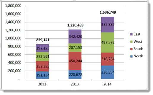
How to Show Percentages in Stacked Bar and Column Charts in Excel

Learn about sensitivity labels - Microsoft Purview Example showing available sensitivity labels in Excel, from the Home tab on the Ribbon. In this example, the applied label displays on the status bar: To apply sensitivity labels, users must be signed in with their Microsoft 365 work or school account. Note For US Government tenants, sensitivity labels are supported for all platforms.

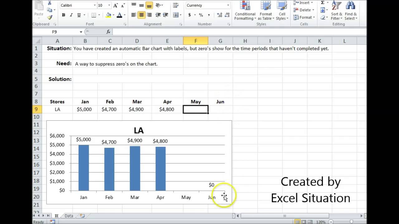
Excel Bar Chart Suppress Zeros - YouTube

50 Excel Shortcuts That You Should Know in 2022 - Simplilearn First, let's create a pivot table using a sales dataset. In the image below you can see that we have a pivot table to summarize the total sales for each subcategory of the product under each category. Fig: Pivot table using sales data 46. To group pivot table items Alt + Shift + Right arrow

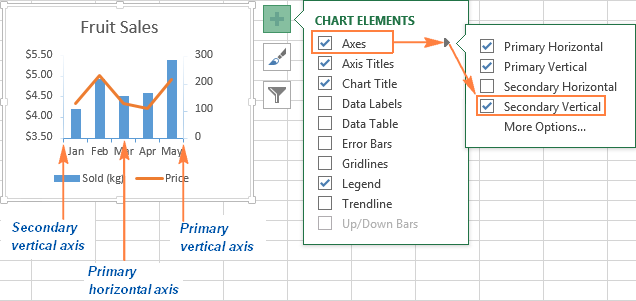
Excel charts: add title, customize chart axis, legend and data labels

Use defined names to automatically update a chart range - Office Select cells A1:B4. On the Insert tab, click a chart, and then click a chart type. Click the Design tab, click the Select Data in the Data group. Under Legend Entries (Series), click Edit. In the Series values box, type =Sheet1!Sales, and then click OK. Under Horizontal (Category) Axis Labels, click Edit.

Charts in Excel - Easy Excel Tutorial

Manage sensitivity labels in Office apps - Microsoft Purview ... Set Use the Sensitivity feature in Office to apply and view sensitivity labels to 0. If you later need to revert this configuration, change the value to 1. You might also need to change this value to 1 if the Sensitivity button isn't displayed on the ribbon as expected. For example, a previous administrator turned this labeling setting off.

CPPTRAJ Manual

Date Axis in Excel Chart is wrong • AuditExcel.co.za In order to do this you just need to force the horizontal axis to treat the values as text by right clicking on the horizontal axis, choose Format Axis Change Axis Type to be Text Note that you immediately lose the scaling options and the date scale puts in exactly what is in the data, onto the horizontal axis.

Creating Pie Chart and Adding/Formatting Data Labels (Excel) - YouTube

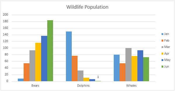
peltiertech.com › select-data-display-in-excelSelect Data to Display in an Excel Chart With Option Buttons Feb 17, 2015 · My suggested approach will add some columns (F:I) to the existing data range with formulas that show or don’t show data based on which of two option buttons is selected, and my chart will use all of this data. When the formulas don’t show the values, they will not appear in the chart. The Data. The extended data range is shown below.

Chart Data Labels in PowerPoint 2011 for Mac

Viewing Data - SAS Tutorials - LibGuides at Kent State University Double-click on the icon of the library where the dataset is located. Locate the dataset icon and double-click on it. This will open your dataset as a spreadsheet. A typical Viewtable view of a dataset looks like this: Note that SAS is unable to execute any DATA or PROC steps on a dataset that is open in the Viewtable window.

Callout Data Labels for Charts in PowerPoint 2013 for Windows

Find Excel column name from a given column number C++ Data Types. Improve Article. Save Article. Like Article. Find Excel column name from a given column number. Difficulty Level : Medium; ... You have experienced while using excel when you see columns and rows numbering are done in Alphabetical ways. Here's How I purposefully think about the logic how it is arranged. (In Mathematical terms ...

Share :